Summary

Machine learning is applied statistics, for the purpose of predicting outcomes for unseen experiences by extrapolating from a set of experiences.

• goal is to minimize generalization error, error incurred when running a model on new testing data, a model that was trained exclusively on a training data set
• overfitting and underfitting are undesirable outcomes of model training, and happen when the capacity of a model is not optimal
  • overfitting is controlled by restricting the hypothesis space, dictating the model's capacity
• in regressions, we have a fixed parameter (weighting) vector
• non-parametric models allow for extreme fitting of data, with a non-fixed parametric vector
• the no free lunch theorem states that the average performance of all classification algorithms over all data sets is equal
• to design a learning algorithm, regularizers are used to specify preference of kinds of functions learned, controlling capacity
• regularization is any modification to the learning algorithm with the intent of reducing generalization error, not training error

Machine Learning Basics

Machine learning is a form of applied statistics, with a lesser emphasis on confidence and greater on statistical estimates.

• Formally, learning is improving a performance measure P, by learning from experience E with respect to some class of tasks T
• in a formal sense, learning is not a task, it is our means of attaining the ability to perform a task
• tasks describe how we should process examples, vectors of quantitative features
  • Classification: specifying one of k categories some input belongs to
  • Classification with missing input: for n inputs, we will need 2^n functions to be learned, for every combination of inputs
  • Regression: based on numeric input, learn a function that can predict outputs outside of the examples
  • Transcription: observe realtively unstructured data, and transcribe it into discrete textual form
  • Machine Translation: language translation (like English to French)
  • Structured Output: any task with vector output (superset of transcription and machine translation)
  • Anomaly Detection: program sifts through a set of events and flags them as being unusual
  • Synthesis: generating new examples, based on the training set
  • Imputation of Missing Values: fill in missing inputs
  • Denoising: for some corrupted example x, and clean example y, find the conditional probability distribution p(y|x)
  • Density estimation (PMF estimation): determine general clustering in a probability mass function
• performance measure is a quantitative measure for an algorithm for success of task T
  • generally test how well it performs on data it hasn't seen, so the test set
• experience is often the dataset, containing features, and in the case of supervised learning it contains annotations with labels or targets

Linear Regression Example

Simple algorithm for solving a regression problem, to predict some scaler y from input vector x in Rn: y = w^Tx, w is a vector n parameters

• w is simply the weights of each xi feature
• set aside a design matrix X^(test) of m examples with a corresponding target vector y^(test) containing correct values of y, not used for training but as performance measure P
  • common performance measure is based on the sum of squared deviation
  • this is minimized when the sum of squared differences function's gradient is 0
  • Mean Square Error is a function of the sum of square differences
  • MSE_test =. 1/m • ∑(ŷ^(test) - y^(test))² from 1 to i
• we want improve weights w to minimize MSE_test, by minimizing MSE_train
• solve for ∇_wMSE_train = 0 the normal equations

Normal Equation is an analytical solution to the linear regression problem, using a least-squares cost function

• starting with: MSE_test =. 1/m • ∑(ŷ^(test) - y^(test))² from 1 to i
• ∇_wMSE_train = 0
• ∇_w 1/m • ∑(ŷ^(test) - y^(test))² = 0
• ∇_w ∑(ŷ^(test) - y^(test))² = 0
• y^(test) = w^Tx is our prediction or hypothesis function for x
• ∇_w ∑(w^Tx - y^(test))² = 0
  • X, the design matrix replaces our summation term, since it represents the m rows of n+1 features, +1 for the intercept
  • use transposed matrix multiplaction (essentially squaring each

Capacity, Overfitting and Underfitting

In machine learning, we want to perform new tasks unseen before, this is called generalization

• one goal is to minimize generalization error, or test error
• generalization error is the expected value of the error for inputs, based on a distribution similar to what real inputs will be
• estimate generaliation error with a test set
• in linear regression, training error is minimized, but we actually care about test error, however you cannot use the test error to affect the result of training since the test error is not part of the training set
• in statistical learning theory, arbitrary collection of examples doesn't allow us to make any adjustments, but assuming data is collected over some probability distribution (data generating process)
  • theoretically, we can follow the i.i.d assumption: independent identically distributed draws
• therefore the test and the train examples are from the same data generating distribution, p_data
  • expected train error = expected test error
• in practice, splitting the sets and minimizing the training error almost certainly means that expected test error ≥ expected train error
  • we want to reduce training error and reduce the gap between training and test error
  • correspond to underfitting and overfitting, and can be mitigated with capacity
• a models capacity is generally it's ability to fit many functions
• high capacity corresponds to overfitting, low to underfitting
• one way to control capacity is to restrict the hypothesis space
  • linear regression models are restricted to the set of linear functions
  • by introducing an x^2 term into the linear regression equation ŷ = b + w1x + w2x² increases the model capacity (increased using more features, x^2, and their corresponding parameters w2)
  • machine learning algorithms work best when they correspond to the appropriate capacity for the true complexity of the task
• in statistical learning theory, model capacity is quantified by the Vapnik-Chervonenkis (VC) dimension
  • measure capacity of binary classifiers
• VC dimension is the largest possible value of m for which there exists a training set of m different x points that the classifier can label arbitrarily
• simpler functions are more likely to generalize (have small difference between training and test error), still need to have sufficient complexity to keep training error low

Non-parametric models allow for high capacity (well fit models)

• non-parametric models are not necessarily bounded by a function (often describe non-practical algorithms)
• linear regression has a fixed length vector of weights, while the nearest neighbour regression (non-parametric) uses X, the training matrix and y, the target vector of corresponding values to each point
  • model looks up the closest training entry to the test point x, and returns the regression target
• non-parametric learning algorithms can be constructed through nested parametric learning algorithms
  • outer algorithm, for learning the number of parameters needed for the inner regression algorithm
• error in mapping x to y can be seen as inherently stochastic or deterministic with non-considered variables
  • the error in a "perfect model" for a given distribution incurs Bayes error
• for non-parametric models, the generalization error decreases with more examples until it reaches the best possible error
• any fixed-parameter model without enough capacity will bound itself to a value greater than Bayes error

The No Free Lunch Theorem

Logically, inferring general rules of a limited set of examples in not valid

• learning theory claims that algorithms can generalize well from a finite training set
  • must have information about every member of the set, otherwise you can't get something from nothing
• learning is based on probabilistic rules rather than logical reasoning
• no free lunch states that every classification algorithm has the same average error over the set of all tasks
  • no learning algorithm is inherently better than any other, without information and assumptions
• important to understand distributions that are relevant to real world experiences and algorithms that work well on data drawn from these data generating distributions

Regularization

The no free lunch theorem implies that the algorithm must be designed well for a task, the only way so far is by changing its capacity (thus affecting the hypothesis space)

• can have more granularity in algorithm design by introducing more kinds of function to the hypothesis space
• modify what we're trying to minimize, by summing the MSE with a criterion, which is pre-defined by the user (λ would control the preference for a preferred function)
• weight decay is an example, where we minimize J(w), second term is just λ • L² norm:

• result is a weighted tradeoff between fitting the training data and being small
• generally, we can regularize a model that learns function f(x;θ) by adding a penalty called a regularizer to the cost function
  • in weight decay, the regularizer Ω(w) = w^Tw
• exclusion from the hypothesis space is infinite preference against it
• to design a learning algorithm, regularizers are used to specify preference of kinds of functions learned, controlling capacity
• regularization is any modification to the learning algorithm with the intent of reducing generalization error, not training error

Hyperparameters

A hyperparameter is not learned by the algorithm, it is predefined like the capacity in a polynomial regression or λ in weight decay

• often parameters that are not easy to optimize (capacity learned from any training set will result in the highest possible capacity, resulting in overfitting)
• a validation set can be formed (partition of the test dataset) to train hyperparameters (over iterations?)
  • after validation set optimizes hyperparameters, generalization error may be estimated with the test set
• cross-validation is the use of all examples in the training and test sets
• k-fold cross-validation partitions the dataset into k non-overlapping subsets, and iterate through each subset as the single test subset, and average the test error across k trials
• when dataset D is too small for simple train/test split to yield accurate estimation of generalization error (mean loss on a small test has high variance)

Estimators, Bias, Variance

Point Estimation attempts to provide the single best prediction

• generally predicting a parameter (or vector of them) e.g. the weights in linear regression
• θ-hat is used to denote an estimator for a parameter θ
• point estimators is just a function of the data,

• Consistency formally describes the probabilistic convergence of a point estimate to the actual value

Maximum Likelihood Estimation

• Maximum Likelihood Estimation helps to formally derive what a good estimator function is for a models
  • we have an unknown distribution, and some sample
  • likelihood of a specific sample coming up is the product of the individual probabilities of each event in the sample
  • now we want to estimate any θ, some parameter of the unknown distribution; let's do the mean
  • then θ-hat is our estimate of θ and it is the selected value of θ for the unknown distribution that maximizes the probability of our sample coming up
• KL Divergence is a measure of non-symmetry between two probability distributions
  • Kullback-Leibler divergence

The MLE can be simplified to finding θ that maximizes the average log likelihood of each event in our sample, the training data.

In ML, the MLE is used to minimize dissimilarity between the empircal distribution of the training set, and the model distribution, as measured by the KL divergence

Conditional Log-Likelihood and MSE

Supervised Learning

Association of some input with some output

• human often acts as "supervisor" annotating data
• many supervised learning algorithms are probabilistic estimating a probability distribution
• using MLE to find best parameter vector

We can generalize linear regression to the classification scenario by defining different families of probability distributions

• in binary classification, we have class 0 and class 1, and combined the probability distributions for both classes should sum to 1 for all domain values
  • since they sum to 1, we only calculate one distribution
• logistical regression: squash a linear regression into the range (0,1) using a logistic sigmoid, and interpret as probability
  • logistic regression is hard, linear regression has optimal weight parameters for its function since there is a closed-form solution
• in logistic regression, we must search for optimal weights by maximizing the log-likelihood funciton, or minimize the negative log-likelihood with gradient descent
  • applies generally to almost all supervised learning problems

Support Vector Machines

Similar to logistic regression, also driven by linear funcition w^Tx + b (weighted vector funciton)

• the goal is similar to logistic regression: find a hyperplane that divides a dataset into two classes
• support vectors are the data points nearest to the hyperplane, if removed would alter the position of the dividing hyperplane
  • margins are the magnitude of the support vectors, and we want to maximize the margins if possible
• while logistic regression provides probabilities, SVMs predict one class for positive output values, and other for negative

Often data doesn't divide nicely. We can approach this by mapping data into a higher dimension:

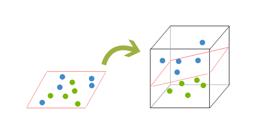
• kernel trick is used to accomplish this -- source
  • applying kernels to improve classification results
  • kernel K(v,w) is a function K: R^N, R^N -> R computing the dot product between v and w
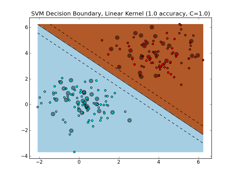
• so a linear SVM finds a hyperplane that best separates data points called the decision boundary
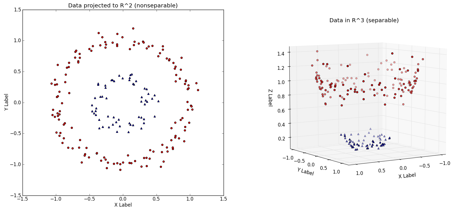
• in most datasets, a linear decision boundary cannot be found in the original feature space/dimensionality
• the challenge in training a linear SVM classifier in finding a decision boundary is that we must apply a good transformation to map the dataset to a higher dimension

We define φ to be a transformation function that maps the dataset X to a higher dimensionality dataset X' (think R2 to R3 as shown above)

• want to train a linear SVM on transformed dataset X' to get a classifier f_SVM
  • after training, during testing, every new example x will first be transformed to x' = φ(x)
• so the output is a label for the class. In otherwords f_SVM(φ(x)) = f_SVM(x') in {0,1} for a binary classification problem
• can achieve nonlinear SVMs by applying linear SVMs in higher dimensions
• this is very simple to understand, but it is also computationally expensive to perform
• we can apply different transformations, one example is a polynomial kernel, and this one maps from R2 -> R5, and by simply transforming the input before performing a linear SVM is extremely expensive in high dimensions

It turns out that SVMs only compute pair-wise dot products and thus we don't need to always work in a higher dimensional space during training/testing

• during the training, the optimization problem only uses pair-wise dot products of examples
• there exists a closed form method to compute dot products in higher dimensions without needing to transform the vectors in the dataset
• kernel functions let us compute this
  • we can implicitly transform datasets to higher dimensional R^M faster and without extra memory
  • in other words, instead of pre-processing data input, then performing dot products, the kernel function can replace dot products and be applied to un-transformed vectors with the same effect
  • the intuition behind this is that the kernel function K can effectively perform a dot product while working exclusively in R^N
• different kernels, or kernel functions, exist to perform dot products in different dimensions with different transformations
  • the chosen dimensional transform is important for finding an effective decision boundary
  • selecting the correct kernel for a task requires a lot of hyperparameter tuning for the model to get good performance
  • K-Fold Cross Validation is a technique that might help